CNNs et computer vision avec PyTorch : Des convolutions à la détection d'objets

10 min de lecture 2118 mots

tl;dr: CNNs = réseaux convolutifs pour vision. Convolution 2D : kernel glisse sur image, détecte patterns (edges→textures→objets). Architecture : Conv2d→ReLU→MaxPool (repeat)→Flatten→Linear. Batch Norm stabilise. ResNet : residual connections = réseaux 100+ couches. Apps : classification, détection (YOLO), segmentation (U-Net).

Les Convolutional Neural Networks (CNNs) ont révolutionné la computer vision en 2012 avec AlexNet. Aujourd’hui, les CNNs sont partout : reconnaissance faciale, voitures autonomes, diagnostic médical, filtres Instagram. Dans cet article, nous allons comprendre les convolutions, implémenter des architectures classiques, et explorer des applications avancées.

Pourquoi les CNNs pour les images ?

Les fully-connected networks (MLPs) ont deux problèmes majeurs avec les images :

Trop de paramètres

# Image 224x224 RGB
image_size = 224 * 224 * 3  # 150,528 pixels

# MLP avec une seule hidden layer de 1000 neurones
fc1 = nn.Linear(150528, 1000)  # 150 millions de paramètres !

Pas de structure spatiale

Les MLPs traitent chaque pixel indépendamment, ignorant que les pixels voisins sont corrélés.

Convolutions

Les convolutions résolvent ces problèmes :

✅ Partage de poids : Même filtre utilisé sur toute l’image
✅ Localité : Chaque neurone regarde seulement une région locale
✅ Invariance de translation : Détecte un pattern partout dans l’image

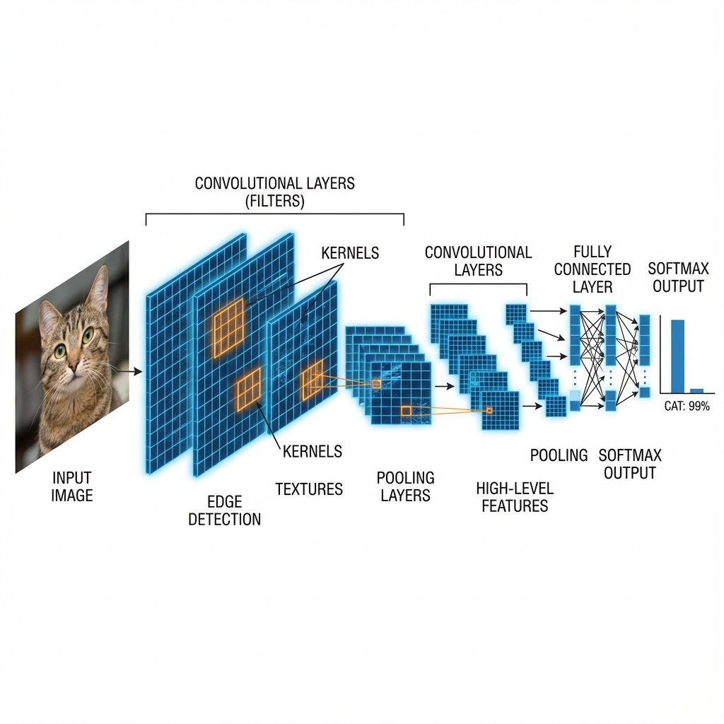
Schéma d’une convolution 2D avec kernel et feature maps

Les convolutions 2D en détail

Opération de convolution

Une convolution applique un kernel (filtre) qui glisse sur l’image :

import torch
import torch.nn as nn

# Convolution 2D simple
conv = nn.Conv2d(
    in_channels=3,      # RGB input
    out_channels=64,    # 64 filtres
    kernel_size=3,      # Kernel 3x3
    stride=1,           # Pas de déplacement
    padding=1,          # Padding pour garder la taille
    bias=True           # Ajouter un biais
)

# Input : batch d'images RGB
x = torch.randn(32, 3, 224, 224)  # (batch, channels, height, width)

# Forward pass
output = conv(x)
print(f"Output shape: {output.shape}")  # (32, 64, 224, 224)

# Paramètres de la convolution
num_params = 3 * 64 * 3 * 3 + 64  # (in × out × k × k) + bias
print(f"Paramètres: {num_params:,}")  # 1,792 params

Formule de la taille de sortie

def conv_output_size(input_size, kernel_size, stride, padding):
    """
    Calcule la taille de sortie d'une convolution
    """
    return (input_size - kernel_size + 2 * padding) // stride + 1

# Exemple
input_h, input_w = 224, 224
kernel_size = 3
stride = 1
padding = 1

output_h = conv_output_size(input_h, kernel_size, stride, padding)
print(f"Output size: {output_h}x{output_w}")  # 224x224

# Sans padding
output_h_no_pad = conv_output_size(224, 3, 1, 0)
print(f"Sans padding: {output_h_no_pad}")  # 222 (perd 2 pixels)

Types de convolutions

# Standard convolution
conv_std = nn.Conv2d(3, 64, kernel_size=3, padding=1)

# Strided convolution (downsampling)
conv_strided = nn.Conv2d(3, 64, kernel_size=3, stride=2, padding=1)
# 224x224 → 112x112

# Large kernel
conv_large = nn.Conv2d(3, 64, kernel_size=7, stride=2, padding=3)
# Réceptive field plus grand

# Dilated (Atrous) convolution
conv_dilated = nn.Conv2d(3, 64, kernel_size=3, padding=2, dilation=2)
# Réceptive field plus grand sans augmenter les paramètres

# Depthwise separable (pour MobileNet)
conv_depthwise = nn.Conv2d(64, 64, kernel_size=3, padding=1, groups=64)
conv_pointwise = nn.Conv2d(64, 128, kernel_size=1)
# Beaucoup moins de paramètres

💡 Padding=1 avec kernel=3 conserve la taille spatiale. Stride=2 divise la taille par 2 (downsampling). Dilation augmente le receptive field sans ajouter de paramètres.

Pooling : Réduction de dimensions

Le pooling réduit la taille spatiale pour :

Diminuer les paramètres
Augmenter le receptive field
Créer une invariance de position

Max pooling

# Max Pooling 2x2
maxpool = nn.MaxPool2d(kernel_size=2, stride=2)

x = torch.randn(32, 64, 224, 224)
output = maxpool(x)
print(f"After maxpool: {output.shape}")  # (32, 64, 112, 112)

# Prend le maximum dans chaque région 2x2
# Exemple :
# [[1, 2],   → max = 4
#  [3, 4]]

Average pooling

# Average Pooling
avgpool = nn.AvgPool2d(kernel_size=2, stride=2)

x = torch.randn(32, 64, 224, 224)
output = avgpool(x)
print(f"After avgpool: {output.shape}")  # (32, 64, 112, 112)

Global average pooling

# Global Average Pooling : H×W → 1×1
gap = nn.AdaptiveAvgPool2d((1, 1))

x = torch.randn(32, 2048, 7, 7)
output = gap(x)
print(f"After GAP: {output.shape}")  # (32, 2048, 1, 1)

# Équivalent à :
# x.mean(dim=[2, 3], keepdim=True)

Architectures CNN classiques

LeNet-5 (1998) : Le pionnier

class LeNet5(nn.Module):
    """
    Architecture originale pour MNIST
    """
    def __init__(self, num_classes=10):
        super().__init__()
        self.conv1 = nn.Conv2d(1, 6, kernel_size=5)
        self.conv2 = nn.Conv2d(6, 16, kernel_size=5)
        self.fc1 = nn.Linear(16 * 5 * 5, 120)
        self.fc2 = nn.Linear(120, 84)
        self.fc3 = nn.Linear(84, num_classes)

    def forward(self, x):
        # Input: (batch, 1, 32, 32)
        x = torch.relu(self.conv1(x))       # → (batch, 6, 28, 28)
        x = torch.max_pool2d(x, 2)          # → (batch, 6, 14, 14)
        x = torch.relu(self.conv2(x))       # → (batch, 16, 10, 10)
        x = torch.max_pool2d(x, 2)          # → (batch, 16, 5, 5)
        x = x.view(x.size(0), -1)           # → (batch, 400)
        x = torch.relu(self.fc1(x))         # → (batch, 120)
        x = torch.relu(self.fc2(x))         # → (batch, 84)
        x = self.fc3(x)                     # → (batch, 10)
        return x

# Test
model = LeNet5()
x = torch.randn(1, 1, 32, 32)
output = model(x)
print(f"Output: {output.shape}")  # (1, 10)

VGGNet (2014) : Profondeur avec petits kernels

class VGGBlock(nn.Module):
    """
    Bloc VGG : N×(Conv3x3 + ReLU) + MaxPool
    """
    def __init__(self, in_channels, out_channels, num_convs):
        super().__init__()
        layers = []
        for _ in range(num_convs):
            layers.append(nn.Conv2d(in_channels, out_channels,
                                   kernel_size=3, padding=1))
            layers.append(nn.ReLU(inplace=True))
            in_channels = out_channels
        layers.append(nn.MaxPool2d(kernel_size=2, stride=2))
        self.block = nn.Sequential(*layers)

    def forward(self, x):
        return self.block(x)

class VGG16(nn.Module):
    """
    VGG16 : 13 conv + 3 fc = 16 layers
    """
    def __init__(self, num_classes=1000):
        super().__init__()
        self.features = nn.Sequential(
            VGGBlock(3, 64, 2),       # 224 → 112
            VGGBlock(64, 128, 2),     # 112 → 56
            VGGBlock(128, 256, 3),    # 56 → 28
            VGGBlock(256, 512, 3),    # 28 → 14
            VGGBlock(512, 512, 3),    # 14 → 7
        )
        self.classifier = nn.Sequential(
            nn.Linear(512 * 7 * 7, 4096),
            nn.ReLU(inplace=True),
            nn.Dropout(0.5),
            nn.Linear(4096, 4096),
            nn.ReLU(inplace=True),
            nn.Dropout(0.5),
            nn.Linear(4096, num_classes)
        )

    def forward(self, x):
        x = self.features(x)               # → (batch, 512, 7, 7)
        x = x.view(x.size(0), -1)          # → (batch, 25088)
        x = self.classifier(x)             # → (batch, num_classes)
        return x

# VGG16 a 138M paramètres !
model = VGG16()
print(f"Params: {sum(p.numel() for p in model.parameters()):,}")

Batch Normalization : Stabiliser l’entraînement

La Batch Normalization normalise les activations pour stabiliser et accélérer l’entraînement.

Principe

# Batch Normalization après convolution
class ConvBNReLU(nn.Module):
    def __init__(self, in_channels, out_channels):
        super().__init__()
        self.conv = nn.Conv2d(in_channels, out_channels,
                             kernel_size=3, padding=1, bias=False)
        # bias=False car BN a son propre biais
        self.bn = nn.BatchNorm2d(out_channels)
        self.relu = nn.ReLU(inplace=True)

    def forward(self, x):
        x = self.conv(x)
        x = self.bn(x)
        x = self.relu(x)
        return x

# Utilisation
block = ConvBNReLU(64, 128)
x = torch.randn(32, 64, 56, 56)
output = block(x)
print(f"Output: {output.shape}")  # (32, 128, 56, 56)

Ordre des opérations

Deux conventions existent :

# Conv → BN → ReLU (plus courant)
nn.Sequential(
    nn.Conv2d(64, 128, 3, padding=1, bias=False),
    nn.BatchNorm2d(128),
    nn.ReLU(inplace=True)
)

# Conv → ReLU → BN (moins courant)
nn.Sequential(
    nn.Conv2d(64, 128, 3, padding=1),
    nn.ReLU(inplace=True),
    nn.BatchNorm2d(128)
)

🔎 Tip
Ordre recommandé : Conv → BN → ReLU est le plus utilisé (ResNet, EfficientNet). Important : Utilisez bias=False dans Conv2d avant BatchNorm (le biais de BN rend celui de Conv inutile).

ResNet : Residual Connections pour Réseaux Profonds

Les réseaux très profonds (>20 couches) souffrent du problème de vanishing gradients. ResNet résout cela avec des skip connections.

Residual block

class ResidualBlock(nn.Module):
    """
    Bloc résiduel de base de ResNet
    """
    def __init__(self, in_channels, out_channels, stride=1):
        super().__init__()
        # Main path
        self.conv1 = nn.Conv2d(in_channels, out_channels,
                              kernel_size=3, stride=stride,
                              padding=1, bias=False)
        self.bn1 = nn.BatchNorm2d(out_channels)
        self.conv2 = nn.Conv2d(out_channels, out_channels,
                              kernel_size=3, padding=1, bias=False)
        self.bn2 = nn.BatchNorm2d(out_channels)

        # Shortcut connection
        self.shortcut = nn.Sequential()
        if stride != 1 or in_channels != out_channels:
            self.shortcut = nn.Sequential(
                nn.Conv2d(in_channels, out_channels,
                         kernel_size=1, stride=stride, bias=False),
                nn.BatchNorm2d(out_channels)
            )

    def forward(self, x):
        identity = x

        # Main path
        out = self.conv1(x)
        out = self.bn1(out)
        out = torch.relu(out)

        out = self.conv2(out)
        out = self.bn2(out)

        # Add skip connection
        out += self.shortcut(identity)
        out = torch.relu(out)

        return out

# Test
block = ResidualBlock(64, 128, stride=2)
x = torch.randn(1, 64, 56, 56)
output = block(x)
print(f"Output: {output.shape}")  # (1, 128, 28, 28)

ResNet complet

class ResNet(nn.Module):
    """
    ResNet simplifié pour CIFAR-10
    """
    def __init__(self, num_classes=10):
        super().__init__()
        self.conv1 = nn.Conv2d(3, 64, kernel_size=3,
                              padding=1, bias=False)
        self.bn1 = nn.BatchNorm2d(64)

        # Residual layers
        self.layer1 = self._make_layer(64, 64, num_blocks=2, stride=1)
        self.layer2 = self._make_layer(64, 128, num_blocks=2, stride=2)
        self.layer3 = self._make_layer(128, 256, num_blocks=2, stride=2)
        self.layer4 = self._make_layer(256, 512, num_blocks=2, stride=2)

        self.avgpool = nn.AdaptiveAvgPool2d((1, 1))
        self.fc = nn.Linear(512, num_classes)

    def _make_layer(self, in_channels, out_channels, num_blocks, stride):
        layers = []
        # Premier bloc avec stride potentiel
        layers.append(ResidualBlock(in_channels, out_channels, stride))
        # Blocs suivants
        for _ in range(1, num_blocks):
            layers.append(ResidualBlock(out_channels, out_channels, stride=1))
        return nn.Sequential(*layers)

    def forward(self, x):
        # Initial conv
        x = self.conv1(x)
        x = self.bn1(x)
        x = torch.relu(x)

        # Residual layers
        x = self.layer1(x)
        x = self.layer2(x)
        x = self.layer3(x)
        x = self.layer4(x)

        # Global pooling + classifier
        x = self.avgpool(x)
        x = x.view(x.size(0), -1)
        x = self.fc(x)

        return x

# Test
model = ResNet(num_classes=10)
x = torch.randn(1, 3, 32, 32)
output = model(x)
print(f"Output: {output.shape}")  # (1, 10)
print(f"Params: {sum(p.numel() for p in model.parameters()):,}")

CNN Moderne : Bloc conv optimal

Le bloc de convolution moderne standard :

class ModernConvBlock(nn.Module):
    """
    Bloc de convolution moderne :
    Conv (bias=False) → BatchNorm → Activation
    """
    def __init__(self, in_channels, out_channels, kernel_size=3,
                 stride=1, padding=1, activation='relu'):
        super().__init__()
        self.conv = nn.Conv2d(
            in_channels, out_channels,
            kernel_size=kernel_size,
            stride=stride,
            padding=padding,
            bias=False  # Pas de biais avant BN
        )
        self.bn = nn.BatchNorm2d(out_channels)

        # Activation
        if activation == 'relu':
            self.act = nn.ReLU(inplace=True)
        elif activation == 'gelu':
            self.act = nn.GELU()
        elif activation == 'silu':  # Swish
            self.act = nn.SiLU(inplace=True)
        else:
            self.act = nn.Identity()

    def forward(self, x):
        x = self.conv(x)
        x = self.bn(x)
        x = self.act(x)
        return x

Visualiser les feature maps

Voir ce que le réseau a appris :

def visualize_feature_maps(model, image, layer_idx=0):
    """
    Visualise les feature maps d'une couche
    """
    import matplotlib.pyplot as plt

    # Hook pour capturer les activations
    activations = []
    def hook(module, input, output):
        activations.append(output.detach())

    # Enregistrer le hook
    handle = list(model.children())[layer_idx].register_forward_hook(hook)

    # Forward pass
    model.eval()
    with torch.no_grad():
        _ = model(image)

    # Retirer le hook
    handle.remove()

    # Visualiser
    feature_maps = activations[0][0]  # Premier exemple du batch
    num_filters = min(64, feature_maps.shape[0])  # Max 64 filtres

    fig, axes = plt.subplots(8, 8, figsize=(12, 12))
    for i, ax in enumerate(axes.flat):
        if i < num_filters:
            ax.imshow(feature_maps[i].cpu(), cmap='viridis')
        ax.axis('off')

    plt.tight_layout()
    plt.savefig('feature_maps.png')
    print(f"Visualized {num_filters} feature maps from layer {layer_idx}")

# Utilisation
# model = ResNet()
# image = torch.randn(1, 3, 224, 224)
# visualize_feature_maps(model, image, layer_idx=1)

Applications Avancées

Classification d’images

# Exemple complet avec ResNet pré-entraîné
from torchvision import models, transforms
from PIL import Image

# Charger modèle
model = models.resnet50(pretrained=True)
model.eval()

# Préparer image
transform = transforms.Compose([
    transforms.Resize(256),
    transforms.CenterCrop(224),
    transforms.ToTensor(),
    transforms.Normalize([0.485, 0.456, 0.406], [0.229, 0.224, 0.225])
])

# Prédire
image = Image.open('cat.jpg')
input_tensor = transform(image).unsqueeze(0)

with torch.no_grad():
    output = model(input_tensor)
    probs = torch.softmax(output, dim=1)
    top5_prob, top5_idx = torch.topk(probs, 5)

print("Top 5 predictions:")
for prob, idx in zip(top5_prob[0], top5_idx[0]):
    print(f"  Class {idx}: {prob:.2%}")

Détection d’objets (Faster R-CNN)

from torchvision.models.detection import fasterrcnn_resnet50_fpn

# Charger modèle de détection pré-entraîné
model = fasterrcnn_resnet50_fpn(pretrained=True)
model.eval()

# Préparer image
image = Image.open('street.jpg')
transform = transforms.ToTensor()
input_tensor = transform(image).unsqueeze(0)

# Détecter objets
with torch.no_grad():
    predictions = model(input_tensor)

# Résultats
boxes = predictions[0]['boxes']      # Bounding boxes
labels = predictions[0]['labels']    # Classes
scores = predictions[0]['scores']    # Confiance

# Filtrer par confiance
threshold = 0.5
for box, label, score in zip(boxes, labels, scores):
    if score > threshold:
        print(f"Detected class {label} with confidence {score:.2f}")
        print(f"  Box: {box.tolist()}")

Segmentation sémantique (DeepLab)

from torchvision.models.segmentation import deeplabv3_resnet50

# Charger modèle de segmentation
model = deeplabv3_resnet50(pretrained=True)
model.eval()

# Préparer image
transform = transforms.Compose([
    transforms.Resize((512, 512)),
    transforms.ToTensor(),
    transforms.Normalize([0.485, 0.456, 0.406], [0.229, 0.224, 0.225])
])

image = Image.open('scene.jpg')
input_tensor = transform(image).unsqueeze(0)

# Segmenter
with torch.no_grad():
    output = model(input_tensor)['out']
    # output: (1, 21, H, W) - 21 classes PASCAL VOC

# Obtenir la classe par pixel
segmentation_mask = output.argmax(1)[0]  # (H, W)

# Visualiser
import matplotlib.pyplot as plt
plt.imshow(segmentation_mask.cpu(), cmap='tab20')
plt.savefig('segmentation.png')

Exercices pratiques

Implémenter VGG11

Créez une version simplifiée de VGG avec 11 couches :

class VGG11(nn.Module):
    def __init__(self, num_classes=10):
        super().__init__()
        # Votre code ici
        # Architecture : [64] → [128] → [256, 256] → [512, 512] → [512, 512]
        # Chaque [] = VGGBlock avec MaxPool
        pass

    def forward(self, x):
        # Votre code ici
        pass

ResNet sur CIFAR-10

Entraînez ResNet sur CIFAR-10 et atteignez >90% accuracy :

# Charger CIFAR-10
# Créer ResNet
# Entraîner avec data augmentation
# Mesurer accuracy sur test set

Visualiser feature maps

Visualisez les feature maps de différentes couches et observez la hiérarchie de features (edges → textures → objets).

Conclusion

Dans cet article, vous avez maîtrisé les CNNs et la computer vision :

✅ Principe des convolutions 2D (kernels, stride, padding)
✅ Pooling (max, average, global average)
✅ Architectures classiques (LeNet, VGG, ResNet)
✅ Batch Normalization pour stabilité
✅ Residual connections pour réseaux profonds
✅ Applications (classification, détection, segmentation)
✅ Visualisation des feature maps

Prochaine étape : Dans le prochain article, nous allons explorer les RNNs, LSTMs et Transformers pour traiter des séquences. Vous apprendrez à gérer des données temporelles et découvrirez l’architecture Transformer qui révolutionne le NLP.

Pour aller plus loin :

Consultez Papers with Code pour les architectures SOTA
Explorez torchvision.models pour plus de modèles
Découvrez notre guide sur le transfer learning pour réutiliser ces architectures

🔎 Tip
Projet pratique : Créez un classifieur d’images custom avec ResNet. Utilisez transfer learning, data augmentation agressive, et visualisez les feature maps. Implémentez aussi la détection d’objets simple avec Faster R-CNN. Objectif : comprendre comment les CNNs extraient des features hiérarchiques !