Optimiser et monitorer son hardware IA pour performances maximales

14 min de lecture 2949 mots

tl;dr: GPU mal configuré = -30-50% performance. Persistence mode NVIDIA élimine 3-5s latence startup. Monitoring continu détecte sous-utilisation (gaspillage $) et throttling (surchauffe). MFU (Model FLOPS Utilization) >40% = bon. Outils : nvidia-smi, Prometheus, Grafana. Optimisations : mixed precision, kernel fusion, batch optimal.

Acheter du hardware IA performant est une chose, en extraire le maximum en est une autre. Un GPU NVIDIA H100 peut théoriquement délivrer 1 979 TFLOPS (FP16), mais en pratique, sans optimisations, on atteint souvent seulement 20-40% de cette puissance.

Enjeux :

Performance : 2-3x speedup avec optimisations appropriées
Coûts : GPU sous-utilisé = argent gaspillé
Fiabilité : Détecter pannes avant downtime
Capacité planning : Anticiper besoins futurs

Cet article vous donnera les outils et techniques pour profiler, optimiser et monitorer votre infrastructure IA.

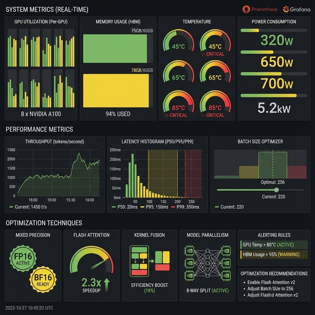
Illustration du matériel et infrastructure pour l’IA : l’optimisation et le monitoring du matériel

Profiling et Diagnostics

Le profiling permet d’identifier les bottlenecks : GPU underutilized, memory bandwidth saturé, CPU idle, etc.

Monitoring GPU avec nvidia-smi

nvidia-smi : Outil de base pour monitoring GPU NVIDIA.

Installation :

# Inclus avec NVIDIA drivers
nvidia-smi

# Version continue (refresh chaque seconde)
nvidia-smi -l 1

# Métriques spécifiques
nvidia-smi --query-gpu=timestamp,name,pci.bus_id,temperature.gpu,utilization.gpu,utilization.memory,memory.total,memory.used,memory.free,power.draw --format=csv -l 1

Exemple output :

+-----------------------------------------------------------------------------+
| NVIDIA-SMI 535.104.05   Driver Version: 535.104.05   CUDA Version: 12.2    |
|-------------------------------+----------------------+----------------------+
| GPU  Name        Persistence-M| Bus-Id        Disp.A | Volatile Uncorr. ECC |
| Fan  Temp  Perf  Pwr:Usage/Cap|         Memory-Usage | GPU-Util  Compute M. |
|===============================+======================+======================|
|   0  NVIDIA H100 80GB    On   | 00000000:01:00.0 Off |                    0 |
| N/A   42C    P0   350W / 700W |  79000MiB / 81920MiB |     95%      Default |
+-------------------------------+----------------------+----------------------+

Métriques clés :

GPU-Util : Utilisation GPU (% du temps avec kernels actifs)
Memory-Usage : VRAM utilisée / totale
Pwr:Usage/Cap : Consommation instantanée / TDP
Temp : Température (< 80°C idéal, > 85°C throttling)
Persistence-M : Mode persistence (On recommandé)

⚠️ Warning
Throttling thermique : Au-delà de 85°C, les GPUs réduisent automatiquement leur fréquence, perdant 10-30% de performance. Surveillez la température et assurez un refroidissement adéquat.

Logs :

# Logger dans fichier
nvidia-smi --query-gpu=timestamp,utilization.gpu,memory.used,temperature.gpu,power.draw --format=csv -l 1 > gpu_log.csv

# Analyser plus tard
python analyze_gpu_usage.py gpu_log.csv

Outils Avancés : nvitop, gpustat

nvitop : Interface interactive améliorée (htop-style).

Installation :

pip install nvitop
nvitop

Features :

Vue multi-GPU élégante
Historique usage (courbes)
Processes par GPU
Alertes visuelles (overtemp, etc.)
Export metrics (JSON, CSV)

gpustat : Vue compacte, parfait pour dashboards.

Installation :

pip install gpustat
gpustat -cp

# Output :
# [0] Tesla V100-SXM2 | 76°C,  95 % | 30000 / 32510 MB | user1(25000M) user2(5000M)

Intégration scripts :

# Watch continu
watch -n 1 gpustat -cp

# JSON pour parsing
gpustat --json

NVIDIA Nsight Systems (Profiling Avancé)

Nsight Systems : Profiler système complet (CPU, GPU, I/O).

Installation :

# Inclus avec CUDA Toolkit
sudo apt install nsight-systems

# Ou download depuis NVIDIA website

Utilisation :

# Profile un script Python
nsys profile -o report python train.py

# Profile avec options détaillées
nsys profile \
  --trace=cuda,nvtx,osrt \
  --sample=cpu \
  --cpuctxsw=true \
  -o profile_output \
  python train.py

Analyse :

# GUI (nécessite X11)
nsys-ui profile_output.nsys-rep

# CLI stats
nsys stats profile_output.nsys-rep

Insights obtenus :

Kernel utilization : Quels kernels CUDA utilisent le plus de temps
Memory transfers : Temps copie CPU ↔ GPU
CPU usage : Bottlenecks data loading
Idle time : GPU idle entre kernels (overhead)

Exemple findings :

- GPU idle 40% du temps → Data loading bottleneck (augmenter num_workers)
- Kernel "matmul" prend 60% du temps → Optimiser avec cuBLAS ou TensorRT
- CPU à 100% → Augmenter DataLoader workers

Profiling PyTorch

PyTorch Profiler : Intégré, facile à utiliser.

Code :

import torch
from torch.profiler import profile, ProfilerActivity, tensorboard_trace_handler

with profile(
    activities=[ProfilerActivity.CPU, ProfilerActivity.CUDA],
    schedule=torch.profiler.schedule(wait=1, warmup=1, active=3, repeat=2),
    on_trace_ready=tensorboard_trace_handler('./log/profiler'),
    record_shapes=True,
    profile_memory=True,
    with_stack=True
) as prof:
    for step, batch in enumerate(dataloader):
        if step >= (1 + 1 + 3) * 2:  # wait + warmup + active * repeat
            break

        outputs = model(batch)
        loss = criterion(outputs, targets)
        loss.backward()
        optimizer.step()
        optimizer.zero_grad()

        prof.step()  # Signal step end

# Visualiser dans TensorBoard
# tensorboard --logdir=./log/profiler

Visualisation TensorBoard :

Timeline : Quand chaque opération s’exécute
Operator view : Temps par type d’opération
Memory view : Allocations mémoire
Kernel view : Kernels CUDA lancés

Diagnostic Mémoire

Identifier memory leaks :

import torch

# Avant training loop
torch.cuda.reset_peak_memory_stats()

# Training loop
for batch in dataloader:
    # ... training code ...

    if step % 100 == 0:
        allocated = torch.cuda.memory_allocated() / 1e9  # GB
        reserved = torch.cuda.memory_reserved() / 1e9
        max_allocated = torch.cuda.max_memory_allocated() / 1e9

        print(f"Step {step}")
        print(f"  Allocated: {allocated:.2f} GB")
        print(f"  Reserved: {reserved:.2f} GB")
        print(f"  Peak: {max_allocated:.2f} GB")

# Si allocated augmente continuellement → memory leak

Memory leak communs :

Tensors non libérés : .detach() oublié
Historique gradients : loss.backward() sans optimizer.zero_grad()
Accumulation tensors : Append dans listes Python

Solution :

# Mauvais
losses = []
for batch in dataloader:
    loss = compute_loss(batch)
    losses.append(loss)  # Garde compute graph !

# Bon
losses = []
for batch in dataloader:
    loss = compute_loss(batch)
    losses.append(loss.item())  # Scalaire Python, pas tensor

Optimisations NVIDIA GPU

Persistence Mode

Problème : Par défaut, NVIDIA driver unload modules quand aucun process n’utilise le GPU. Au prochain lancement, 3-5s d’initialisation.

Solution : Persistence mode garde le driver chargé.

Activation :

# Activer (root requis)
sudo nvidia-smi -pm 1

# Vérifier
nvidia-smi | grep Persistence-M
# Persistence-M| Bus-Id  → On

# Désactiver
sudo nvidia-smi -pm 0

🔎 Tip
Gain immédiat : Le persistence mode élimine 3-5s de latence au démarrage de chaque job. Pour des workloads fréquents ou du serving production, cette optimisation simple est essentielle.

Impact :

Élimination 3-5s latency au lancement
Monitoring nvidia-smi instantané
Recommandé pour serveurs production et calculs ROI

Persistance après reboot :

# Systemd service
sudo nvidia-persistenced

# Activer au boot
sudo systemctl enable nvidia-persistenced

Power Limit Tuning

Principe : Ajuster le TDP pour optimiser performance/consommation.

Use cases :

Undervolting : Réduire TDP pour économie énergie (perte perf minime)
Overclocking : Augmenter TDP (si refroidissement adéquat)

Exemple : RTX 4090 (TDP 450W)

# Voir power limits
nvidia-smi -q -d POWER

# Power Limit          : 450.00 W
# Default Power Limit  : 450.00 W
# Min Power Limit      : 100.00 W
# Max Power Limit      : 600.00 W

# Réduire à 350W (économie énergie)
sudo nvidia-smi -pl 350

# Reset au défaut
sudo nvidia-smi -pl 450

Impact undervolting (350W vs 450W) :

Performance : -5 à -10%
Consommation : -22%
Température : -8°C
Bruit : -15%

Courbe efficiency :

Performance
100% ┤     ╱──────  450W (TDP max)
     │   ╱──
 95% ┤ ╱── 350W (sweet spot)
     │╱
 80% ┼── 250W
     │
     └──────────────────> Consommation

Recommandation : Tester 350-400W pour RTX 4090 (excellent compromis).

Clock Tuning (Overclocking)

Attention : Overclocking annule garantie et augmente usure. Réservé utilisateurs avancés.

Outil : nvidia-settings (Linux GUI) ou MSI Afterburner (Windows)

Linux CLI :

# Autoriser overclocking
sudo nvidia-xconfig --cool-bits=28
# (Reboot requis)

# Voir clocks actuelles
nvidia-smi -q -d CLOCK

# Augmenter core clock (+100 MHz)
nvidia-settings -a "[gpu:0]/GPUGraphicsClockOffset[3]=100"

# Augmenter memory clock (+500 MHz)
nvidia-settings -a "[gpu:0]/GPUMemoryTransferRateOffset[3]=500"

Benchmarking :

# Avant OC
python benchmark.py
# LLaMA 7B: 120 tokens/s

# Après OC (+100 core, +500 mem)
python benchmark.py
# LLaMA 7B: 135 tokens/s (+12%)

Risques :

Instabilité : Crashes, corruptions mémoire
Chaleur : Throttling si cooling insuffisant
Usure : Durée de vie réduite

Recommandation : Ne pas OC en production. OK pour benchmarking/recherche.

MIG (Multi-Instance GPU)

MIG (Multi-Instance GPU) : Partitionner un A100/H100 en plusieurs GPU virtuels indépendants.

Disponible sur : A100, A30, H100, H200

Use cases :

Multi-tenants : Plusieurs équipes partagent un GPU
Isolation : Garantir ressources (QoS)
Cost efficiency : Utiliser 100% du GPU pour optimiser le budget hardware

Modes MIG :

GPU	Profils MIG Disponibles
A100 40GB	1×7g.40gb, 2×3g.20gb, 3×2g.20gb, 7×1g.5gb
A100 80GB	1×7g.80gb, 2×3g.40gb, 3×2g.20gb, 7×1g.10gb
H100 80GB	1×7g.80gb, 2×3g.40gb, 3×2g.20gb, 7×1g.10gb

g = compute units (GPU slices), GB = mémoire

Activation :

# Activer MIG mode
sudo nvidia-smi -mig 1

# Créer 2 instances 3g.40gb (A100 80GB)
sudo nvidia-smi mig -cgi 3g.40gb,3g.40gb -C

# Lister instances
nvidia-smi mig -lgi

# +-----------------------------------------------------------------------------+
# | MIG devices:                                                                |
# +------------------+----------------------+-----------+-----------------------+
# | GPU  GI  CI  MIG |         Memory-Usage |        Vol|         Shared        |
# |      ID  ID  Dev |           BAR1-Usage |     SM    |      Unc. ECC         |
# |================================================================================
# |  0    0   0   0  |     10MiB / 40960MiB | 42      0 |                  0    |
# |                  |      0MiB / 65535MiB |           |                       |
# +------------------+----------------------+-----------+-----------------------+
# |  0    1   0   1  |     10MiB / 40960MiB | 42      0 |                  0    |
# |                  |      0MiB / 65535MiB |           |                       |
# +------------------+----------------------+-----------+-----------------------+

Utilisation :

# Assigner process à MIG instance 0
CUDA_VISIBLE_DEVICES=MIG-<UUID-instance-0> python train.py

# Ou
nvidia-smi mig -lgip  # Lister UUIDs

Avantages :

Isolation forte : Erreur un tenant n’affecte pas les autres
QoS : Garantie ressources
Billing : Facturation fine par instance

Limites :

Performance légèrement inférieure vs GPU entier (overhead)
Pas de NVLink entre instances
Configuration statique (pas de resize dynamique)

CUDA Graphs

Problème : Lancer kernels CUDA a un overhead (~10-20 μs par kernel). Pour petits kernels, overhead > compute !

Solution : CUDA Graphs capture la séquence de kernels et la relance en un seul appel.

Speedup : 10-30% pour modèles avec nombreux petits kernels.

PyTorch :

import torch

# Model, optimizer setup
model = ...
optimizer = ...

# Warmup (CUDA graphs nécessite exécution préalable)
for _ in range(3):
    outputs = model(input)
    loss = criterion(outputs, targets)
    loss.backward()
    optimizer.step()
    optimizer.zero_grad()

# Capture graph
g = torch.cuda.CUDAGraph()
optimizer.zero_grad(set_to_none=True)

with torch.cuda.graph(g):
    static_output = model(static_input)
    static_loss = criterion(static_output, static_targets)
    static_loss.backward()
    optimizer.step()

# Training loop
for inputs, targets in dataloader:
    # Copier données vers static tensors
    static_input.copy_(inputs)
    static_targets.copy_(targets)

    # Replay graph (très rapide)
    g.replay()

Limites :

Shapes tenseurs doivent être fixes (pas de dynamic shapes)
Pas de CPU sync dans le graph
Debugging plus difficile

Use cases :

Inférence (shapes fixes)
Training avec batch size constant

Optimisation Multi-GPU

Data Parallel (DP) vs Distributed Data Parallel (DDP)

Data Parallelism : Répliquer modèle sur chaque GPU, diviser batch.

DataParallel (DP) : PyTorch legacy, single-process

import torch.nn as nn

model = nn.DataParallel(model, device_ids=[0, 1, 2, 3])

Problèmes DP :

Single-process → GIL Python limite
GPU 0 overload (aggregation)
Inefficace (30-50% scaling loss)

DistributedDataParallel (DDP) : PyTorch moderne, multi-process

import torch.distributed as dist
from torch.nn.parallel import DistributedDataParallel as DDP

# Init process group
dist.init_process_group(backend='nccl')

# Model to DDP
model = model.to(rank)  # rank = GPU ID
model = DDP(model, device_ids=[rank])

# Training loop identique

Lancement :

# torchrun (PyTorch 1.10+)
torchrun --nproc_per_node=4 train_ddp.py

# Ou python -m torch.distributed.launch (legacy)
python -m torch.distributed.launch --nproc_per_node=4 train_ddp.py

Scaling DDP : 90-95% efficiency sur 4-8 GPUs (vs 50-70% DP)

NCCL Tuning

NCCL (NVIDIA Collective Communications Library) : Backend communication DDP.

Variables d’environnement :

# Algorithmes optimisés
export NCCL_ALGO=Tree  # Ou Ring (tester les deux)

# Protocole (InfiniBand ou IP)
export NCCL_SOCKET_IFNAME=eth0  # Interface réseau
export NCCL_IB_DISABLE=1  # Désactiver InfiniBand si pas dispo

# Debugging
export NCCL_DEBUG=INFO  # Logs verbeux
export NCCL_DEBUG_SUBSYS=ALL

# Performance tuning
export NCCL_P2P_DISABLE=0  # Activer P2P (NVLink)
export NCCL_SHM_DISABLE=0  # Shared memory

Benchmarking NCCL :

# NCCL Tests (officiel NVIDIA)
git clone https://github.com/NVIDIA/nccl-tests.git
cd nccl-tests
make

# All-reduce benchmark (typique DDP)
./build/all_reduce_perf -b 8 -e 1G -f 2 -g 4

# Output :
#       size    count    time   algbw   busbw
#        8MB     2.0K   500us  16.0GB/s  30.0GB/s
#       16MB     1.0K   900us  17.8GB/s  33.3GB/s

Targets (NVLink) :

2 GPUs : 50 GB/s
4 GPUs : 100 GB/s
8 GPUs : 150 GB/s

Gradient Accumulation

Use case : Simuler large batch size avec GPU limités.

Principe :

# Batch effectif = batch_size × accumulation_steps
# Exemple : 4 × 8 = 32 (comme si batch 32 sur 1 GPU)

model.zero_grad()

for i, (inputs, targets) in enumerate(dataloader):
    outputs = model(inputs)
    loss = criterion(outputs, targets) / accumulation_steps
    loss.backward()

    if (i + 1) % accumulation_steps == 0:
        optimizer.step()
        model.zero_grad()

Avantages :

Large batch sans OOM
Stabilité training (large batch)

Inconvénients :

Temps/epoch multiplié par accumulation_steps
Batch norm peut être affecté

Benchmarking

Synthetic Benchmarks

PyTorch Benchmark :

import torch
import time

def benchmark_matmul(size=8192, iterations=100, warmup=10):
    a = torch.randn(size, size, device='cuda')
    b = torch.randn(size, size, device='cuda')

    # Warmup
    for _ in range(warmup):
        c = torch.matmul(a, b)

    torch.cuda.synchronize()
    start = time.time()

    for _ in range(iterations):
        c = torch.matmul(a, b)

    torch.cuda.synchronize()
    elapsed = time.time() - start

    # TFLOPS calculation
    flops = 2 * size**3 * iterations  # matmul = 2*N³ FLOPS
    tflops = flops / elapsed / 1e12

    print(f"Matrix size: {size}x{size}")
    print(f"Time: {elapsed:.2f}s")
    print(f"Performance: {tflops:.2f} TFLOPS")

benchmark_matmul()

💡 Performance théorique vs réelle : Un H100 délivre 1 979 TFLOPS théoriques (FP16) mais seulement 40-60% en pratique (MFU). Comparez vos benchmarks à ces valeurs pour identifier les sous-performances et optimiser votre ROI hardware.

Targets (FP32 matmul) :

RTX 4090 : 82 TFLOPS
A100 : 156 TFLOPS (SXM), 19,5 TFLOPS (base)
H100 : 67 TFLOPS (FP32), 1 979 TFLOPS (FP16 Tensor Cores)

MLPerf

MLPerf : Benchmark standard industrie (training & inference).

Catégories :

Training : ResNet-50, BERT, GPT-3
Inference : Latence, throughput, offline, server

Utilisation :

# Clone repo
git clone https://github.com/mlcommons/training_results_v3.0.git

# Run benchmark (exemple ResNet-50)
cd training_results_v3.0/NVIDIA/benchmarks/resnet/implementations/pytorch
python train.py --config config_DGXA100.sh

Résultats publics : https://mlcommons.org/benchmarks/training/

Comparaison :

Votre setup vs SOTA (State of the Art)
Identifier sous-performance

Model FLOPS Utilization (MFU)

MFU : Métrique clé pour évaluer efficiency.

Formule :

MFU = FLOPS achieved / FLOPS peak

Exemple : LLaMA 7B training, H100
- FLOPS achieved : 800 TFLOPS
- FLOPS peak H100 : 1 979 TFLOPS (FP16 Tensor Cores)
- MFU : 800 / 1979 = 40%

Targets :

< 20% : Mal optimisé (bottlenecks majeurs)
20-40% : Acceptable
40-60% : Bon (typique LLM training bien optimisé)
> 60% : Excellent (rare, nécessite optimisations poussées)

🔎 Tip
MFU > 40% = optimisation réussie : Un MFU supérieur à 40% indique une bonne utilisation du hardware. En dessous de 20%, recherchez les bottlenecks (data loading, CPU, memory bandwidth).

Calcul automatique :

import torch

def calculate_mfu(model, gpu_name="H100", dtype=torch.float16):
    # FLOPS peak GPU (dict)
    peak_flops = {
        "H100": 1979e12,  # FP16 Tensor Cores
        "A100": 312e12,
        "RTX_4090": 660e12,
    }

    # Mesurer FLOPS achieved
    # (Utiliser profiler ou estimation théorique)
    flops_achieved = measure_flops(model)  # Votre méthode

    mfu = flops_achieved / peak_flops[gpu_name]
    return mfu

print(f"MFU: {calculate_mfu(model) * 100:.1f}%")

Monitoring Continu (Production)

Prometheus + Grafana Stack

Architecture :

[GPU Servers] → [Exporters] → [Prometheus] → [Grafana]
                                  ↓
                            [Alertmanager]

Installation Prometheus :

# Download
wget https://github.com/prometheus/prometheus/releases/download/v2.45.0/prometheus-2.45.0.linux-amd64.tar.gz
tar xvf prometheus-2.45.0.linux-amd64.tar.gz
cd prometheus-2.45.0.linux-amd64

# Config prometheus.yml
cat > prometheus.yml <<EOF
global:
  scrape_interval: 15s

scrape_configs:
  - job_name: 'gpu-servers'
    static_configs:
      - targets:
        - 'localhost:9100'  # node_exporter
        - 'localhost:9445'  # dcgm-exporter
EOF

# Run
./prometheus --config.file=prometheus.yml

DCGM Exporter (NVIDIA)

DCGM (Data Center GPU Manager) : Monitoring GPU avancé pour datacenter.

Installation :

# Docker (recommandé)
docker run -d --gpus all --rm \
  -p 9445:9445 \
  nvcr.io/nvidia/k8s/dcgm-exporter:3.1.7-3.1.4-ubuntu20.04

Métriques exportées (100+ métriques) :

GPU utilization, memory usage
Temperature, power draw
PCIe throughput, NVLink bandwidth
ECC errors, throttling events
Compute processes

Prometheus scrape :

# prometheus.yml
scrape_configs:
  - job_name: 'dcgm'
    static_configs:
      - targets: ['localhost:9445']

Grafana Dashboards

Installation Grafana :

# Ubuntu/Debian
sudo apt install -y software-properties-common
sudo add-apt-repository "deb https://packages.grafana.com/oss/deb stable main"
wget -q -O - https://packages.grafana.com/gpg.key | sudo apt-key add -
sudo apt update && sudo apt install grafana

# Start
sudo systemctl start grafana-server
sudo systemctl enable grafana-server

# Access : http://localhost:3000 (admin/admin)

Dashboards GPU :

Importez dashboard ID 12239 (NVIDIA DCGM Exporter)
Ou créez custom dashboard

Exemple panels :

GPU Utilization (gauge, 0-100%)
VRAM Usage (graph, timeline)
Temperature (graph, alerte si > 85°C)
Power Draw (graph)
Throughput (samples/sec, custom metric)

Alertes Grafana :

# Alert : GPU underutilized
- alert: GPUUnderutilized
  expr: DCGM_FI_DEV_GPU_UTIL < 10
  for: 10m
  annotations:
    summary: "GPU {{ $labels.gpu }} underutilized ({{ $value }}%)"

# Alert : GPU overheating
- alert: GPUOverheating
  expr: DCGM_FI_DEV_GPU_TEMP > 85
  for: 5m
  annotations:
    summary: "GPU {{ $labels.gpu }} temp {{ $value }}°C"

Custom Metrics (Application-Level)

Instrumenter le code :

from prometheus_client import Counter, Histogram, Gauge, start_http_server

# Métriques custom
inference_requests = Counter('inference_requests_total', 'Total inference requests')
inference_latency = Histogram('inference_latency_seconds', 'Inference latency')
gpu_memory_used = Gauge('gpu_memory_used_bytes', 'GPU memory used', ['gpu_id'])

# Start Prometheus endpoint
start_http_server(8000)

# Dans le code
@inference_latency.time()
def run_inference(input):
    inference_requests.inc()
    output = model(input)

    # Update GPU memory
    gpu_memory_used.labels(gpu_id='0').set(torch.cuda.memory_allocated())

    return output

Scrape custom metrics :

# prometheus.yml
scrape_configs:
  - job_name: 'ml-app'
    static_configs:
      - targets: ['localhost:8000']

Dashboards Exemple

Dashboard “GPU Health” :

Row 1: GPU Utilization (tous GPUs, gauge)
Row 2: VRAM Usage (graph, par GPU)
Row 3: Temperature (heatmap, tous GPUs)
Row 4: Power Draw (graph)
Row 5: Processes (table, top 10 par GPU)

Dashboard “Training Monitoring” :

Row 1: Loss (graph, log scale)
Row 2: Throughput (samples/s, graph)
Row 3: Learning Rate (graph)
Row 4: GPU Utilization (graph)
Row 5: Memory Usage (graph, allocated vs reserved)

Checklist Optimisation

Avant de déclarer “mon GPU est lent” :

✅ Configuration système :

Persistence mode activé (nvidia-smi -pm 1)
Power limit approprié (pas en mode eco par erreur)
Pas de throttling thermique (temp < 85°C)
Drivers récents (12 mois max)
CUDA / cuDNN compatibles

✅ Code :

Batch size maximal (fill VRAM à 90%)
Mixed precision activée (FP16/BF16)
DataLoader num_workers optimisé (4-8 typique)
Gradient checkpointing si VRAM limite (voir fine-tuning)
Pas de syncs CPU inutiles (torch.cuda.synchronize())
Tensors sur GPU (pas CPU ↔ GPU copies répétées)

✅ Multi-GPU :

DDP (pas DP)
NCCL configuré (NVLink actif)
Gradient accumulation si small batch

✅ Monitoring :

GPU utilization > 80% (sinon bottleneck data/CPU)
Memory usage > 70% (sinon batch size trop petit, considérer quantization)
MFU > 30% (sinon optimiser compute avec vLLM pour l’inférence)

Conclusion

L’optimisation et le monitoring sont cruciaux pour rentabiliser votre hardware IA. Un GPU H100 à 40% MFU est un gaspillage de 210 000€ de performance potentielle.

Points clés :

Profiling : Identifier bottlenecks avant d’optimiser aveuglément
GPU config : Persistence mode, power tuning, MIG si multi-tenant
Code : DDP, mixed precision, batch size optimal
Monitoring : Prometheus + Grafana pour surveillance 24/7 en production
MFU : Viser > 40% pour LLM training

Gains typiques :

Persistence mode : -3s latency démarrage
Mixed precision : +2x speedup
DDP vs DP : +40% scaling efficiency
Power tuning : -20% consommation, -5% perf
Batch size optimal : +30% throughput

Prochain article : Nous comparerons les offres cloud (AWS, GCP, Azure, Lambda Labs) pour le hardware IA, avec benchmarks de prix et performances.